The Mathematics Behind Transformer Models

Transformer models are now a cornerstone in natural language processing (NLP) and machine learning. They've led to remarkable advancements such as GPT, BERT, and T5 which have demonstrated unprecedented capabilities in 'understanding' and manipulating human language, largely due to their unique architecture that integrates self-attention mechanisms, positional encodings, and deep learning principles.

Part One: Word Embeddings

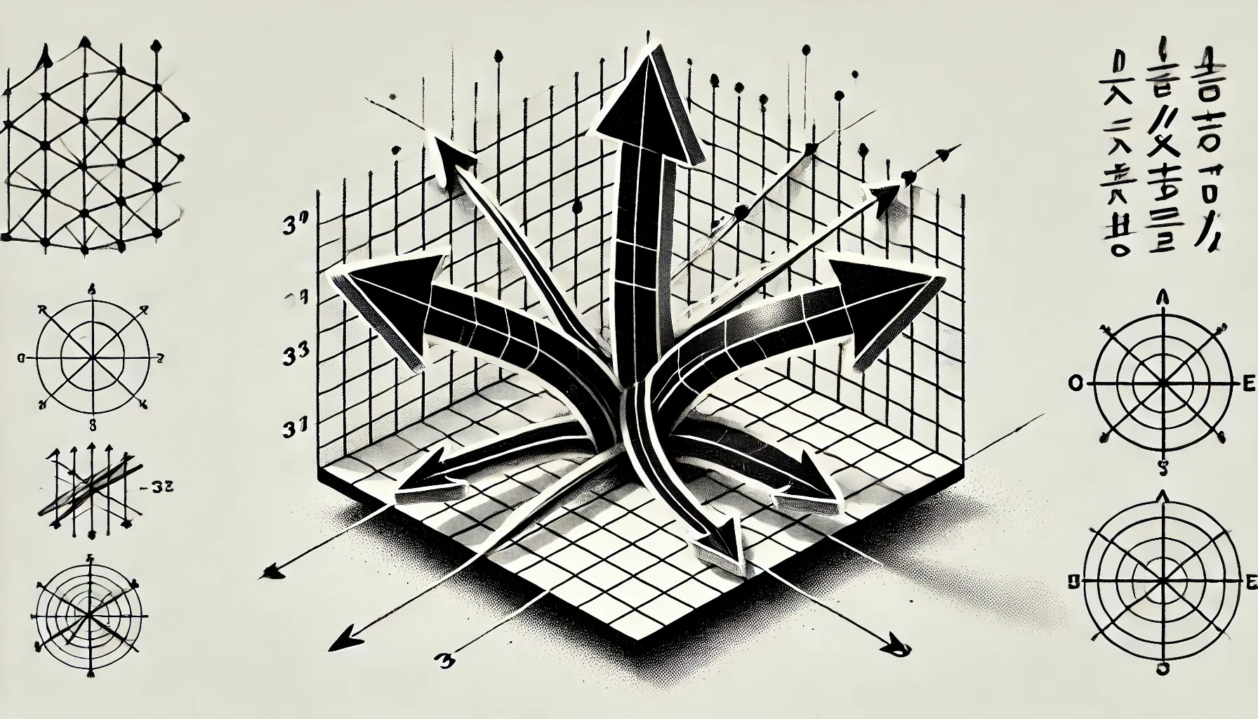
When we think of a word we think of its meaning and maybe any connotations it has. This is exactly how a machine learning model thinks of a word, except words are somehow represented through neuron firings in our brain and digitally in an ML model. The first step in any model dealing with words involves converting words into numerical vectors, a process known as word embedding. Words in their raw text form can't be processed directly by machine learning algorithms so they are transformed into these continuous-valued vectors that capture both syntactic (the arrangement and order of words in a sentence or phrase according to the rules of grammar) and semantic (the actual meaning or interpretation of a word) meanings.

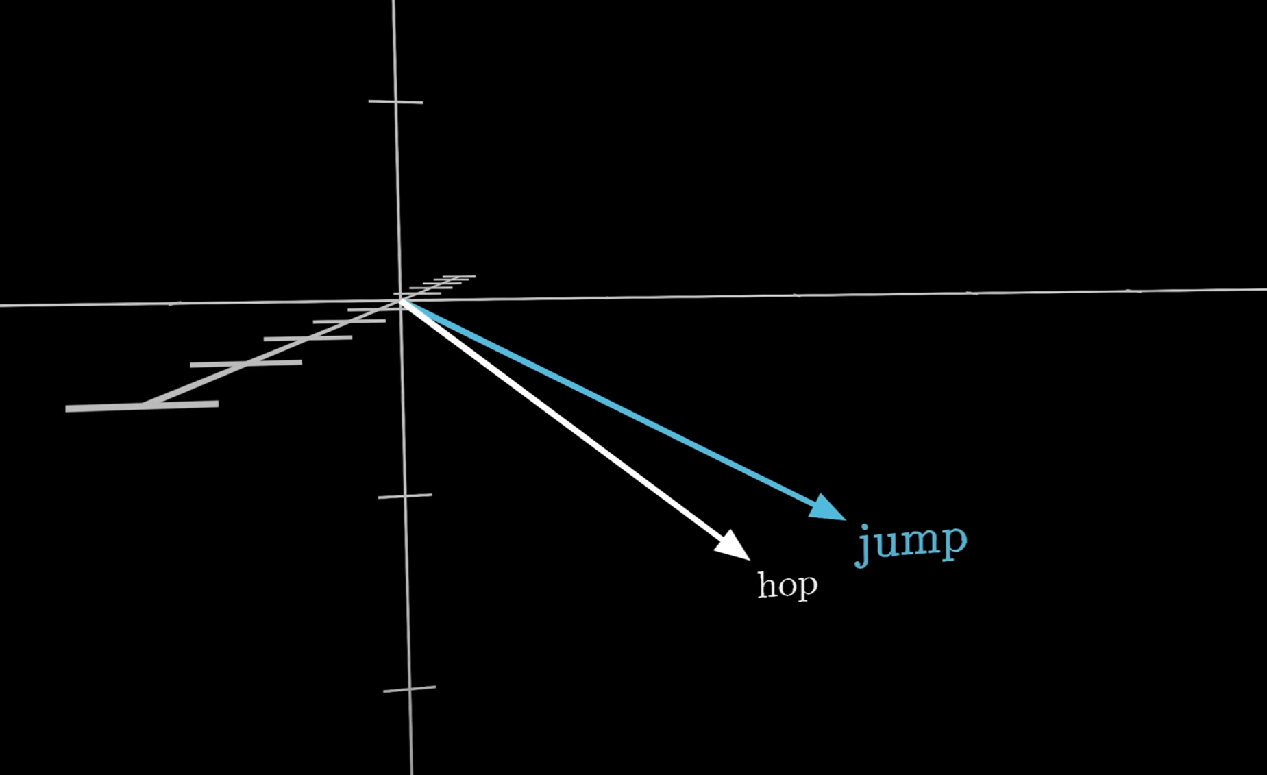
This works so that words with similar meanings or with close relation to each other are physically closer to each other (as visualised in the image above).

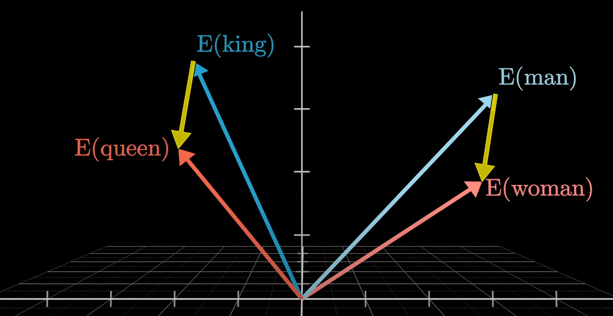
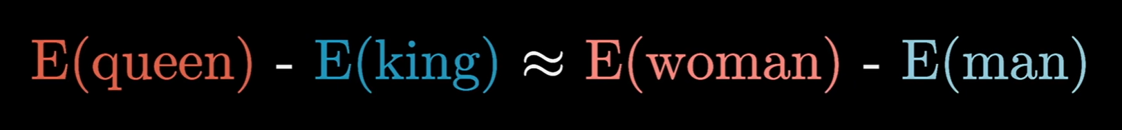
Each dimension of the vector represents a unique aspect of the word. To take a simplistic example we could consider the words man and woman. In the visualisation below you can see that the difference in vector space between the words man and woman is the same as the difference between the words king and queen. The intuitive interpretation of this is that the dimension (direction) that changes by the magnitude of the grey arrow represents masculinity/femininity such that a more feminine "man" = a "woman" and a more feminine "king" = a "queen".

Given a vocabulary of size \( V \) and an embedding dimension \( d \), we can represent this transformation using an embedding matrix \( E \in \mathbb{R}^{V \times d} \). For a word \( w_i \), its embedding \( x_i \) can be defined as:

$$x_i = E(w_i) \in \mathbb{R}^d$$

For example, if you relate this expression to the visualisation above:

These embeddings are learned from a lot of (text) data, where the context of words is used to shape their vector representations. This step is fundamental because it allows the model to handle words as points in a high-dimensional space, making them suitable for neural network processing.

Part Two: Attention

A fundamental innovation of the transformer architecture is the self-attention mechanism. This is what allows each word (in a sequence of words) to pay attention to (or, more accurately, 'attend' to) all the other words. What this does is allow the model to understand dependencies and relationships between words, importantly regardless of the distance between them in the input sequence.

To explain this, I must first introduce the concepts of the query (Q), key (K), and value (V) matrices. These matrices are linear transformations of the input embeddings:

$$Q = XW^Q, \quad K = XW^K, \quad V = XW^V$$

where \( X \in \mathbb{R}^{n \times d} \) is the matrix of input word embeddings for a sequence of length \( n \), and \( W^Q, W^K, W^V \in \mathbb{R}^{d \times d_k} \) are learned weight matrices.

But what are these learned weight matrices? Well, these are a bunch of weights which you can think of as knobs which the model, when training, can turn to influence its output. Therefore a learned weight matrix is one which has gone through training and then is used to create a given output.

These query, key and value matrices are then used to calculate the attention scores, which determine how much attention each word should give to all the other words. They are calculated using the dot product of the query and key matrices. This result is scaled by \( \frac{1}{\sqrt{d_k}} \) for numerical stability (to keep the numbers from getting too big):

$$\text{Attention}(Q, K, V) = \text{softmax}\left(\frac{QK^T}{\sqrt{d_k}}\right)V$$

After that, a function called softmax is applied which normalises the matrix of attention scores and turns them into probabilities that sum to one. This is a super intuitive step where the highest scores get the highest probability and it also reduces the impact of lower scores, allowing the model to focus more on the highest probability (and therefore more relevant) words.

Part Three: Multi-Head

To enhance the model's capacity to capture different types of relationships between words, the transformer uses multi-head attention. This approach involves running several self-attention layers (heads) in parallel. Each head operates with its own \( Q \), \( K \), and \( V \) matrices which allows the model to look at a sentence from lots of different angles at the same time; where each head pays attention to different parts of the sentence or different relationships between words.

The output of each head \( i \) is computed as:

$$\text{head}_i = \text{Attention}(Q_i, K_i, V_i)$$

These outputs are then concatenated and linearly transformed to form the final output of the multi-head attention layer:

$$\text{MultiHead}(Q, K, V) = \text{Concat}(\text{head}_1, \ldots, \text{head}_h)W^O$$

where \( W^O \in \mathbb{R}^{hd_k \times d} \) is a learned weight matrix.

Using the multi-head attention mechanism allows the model to learn and understand different types of relationships and patterns in the input data more effectively. It also improves understanding of complex patterns along with better understanding of context. Additionally, if you want to increase model capacity, instead of increasing the size of a single attention layer you can have lots of smaller heads which will allow the model to learn more complex features without significant increase in computation cost!

Part Four: Positional Encoding

Unlike recurrent neural networks (RNNs), transformers lack an inherent notion of word order. To address this, positional encodings are added to the input embeddings to inform the model about the position of each word in the sequence.

A common method for positional encoding involves using sinusoidal functions:

\[\text{PE}_{(pos, 2i)} = \sin\left(\frac{pos}{10000^{\frac{2i}{d}}}\right), \quad \text{PE}_{(pos, 2i+1)} = \cos\left(\frac{pos}{10000^{\frac{2i}{d}}}\right)\]

where \( pos \) represents the position in the sequence and \( i \) the dimension. Importantly, these sinusoidal patterns allow the model to differentiate between words based on their positions whilst still preserving relative distances.

Part Five: Feed-Forward Networks

After the attention mechanism, each word representation passes through a feed-forward network (FFN) which involves two linear transformations with a ReLU activation in between:

$$\text{FFN}(x) = \max(0, xW_1 + b_1)W_2 + b_2$$

where \( W_1 \in \mathbb{R}^{d \times d_{\text{ff}}} \) and \( W_2 \in \mathbb{R}^{d_{\text{ff}} \times d} \) are learned weight matrices, and \( b_1 \) and \( b_2 \) are biases. The FFN is applied to each position independently and identically, introducing non-linearities that help the model capture complex patterns in the data. This is because introducing these non-linearities breaks the linear limitations that would limit the model's ability to understand any complex patterns that weren't linear - a super important step as so much real-world data like language, images etc. are highly non-linear.

The non-linear activation function (like ReLU, sigmoid or tanh) in the FFN allow the model to combine input features in more intricate ways. They do this by transforming their input in non-linear ways (i.e. a bend or curve) which allow them to model more complex relationships. This is important to introduce more non-linear functions, as stated before, to capture more complex patterns.

Why ReLU?

ReLU looks like the following:

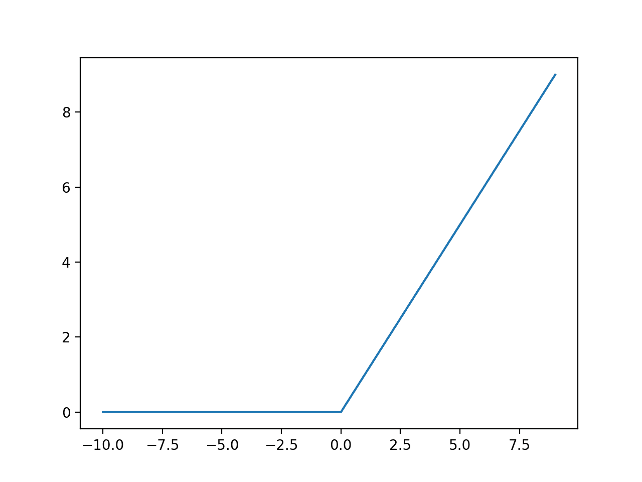
where the function outputs zero for negative inputs and keeps positive inputs the same.

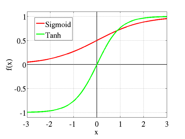
It's quite simple but actually works very well in practice because it avoids the vanishing gradient problem which can be caused by other activation functions like sigmoid and tanh which can 'squash' values into a narrow range, causing gradients to become very small and slowing down the model's learning speed. ReLU does not compress positive values which therefore helps maintain larger gradients during backpropagation, allowing the model to learn faster and more effectively.

It also has sparse activation as it outputs zero for negative values, meaning it only activates some neurons at a time. Sparsity, like this, can lead to more efficient computation and reduce the likelihood of overfitting as not all neurons are active simultaneously.

For positive inputs ReLU behaves like a linear function which actually is beneficial for very large values which are then not saturated, allowing the model to propagate gradients without much distortion.

Interestingly, ReLU is somewhat inspired by biological neuron firings as biological neurons are either activated or not, rather than a smooth curve of activation like sigmoid or tanh. (Not really an advantage just a reason for why it was a popular function to start with). It is also very simple and easy to implement which makes it computationally efficient and speeds up training significantly compared to other activation functions.

Part Six: Stabilisation and Optimisation

To stabilise training and make optimisation more efficient, transformers use layer normalization and residual connections.

Layer Normalisation

Layer normalisation helps stabilise the training of the model by keeping a consistent range of values being fed into each input layer. To do this it calculates the mean and variance of the values in the input and then adjusts the input so that it has a mean of 0 and variance of 1:

$$\text{LN}(x) = \frac{x - \mu}{\sqrt{\sigma^2 + \epsilon}}$$

where \( x \) is the input, \( \mu \) and \( \sigma^2 \) are the mean and variance of the input, and \( \epsilon \) is a small constant for numerical stability.

Residual Connections

Residual connections are like shortcuts which can skip layers (can be more than one) in the network, allowing the input to pass through without any big changes. This allows gradients to flow through the network without diminishing, preventing the 'vanishing gradient' problem: when a gradient gets very small it can 'vanish' which makes learning really difficult.

Residual connections work by adding the original input \( x \) to the output of a sublayer (like multi-head attention or a FFN) and then normalising it:

$$\text{Output} = \text{LayerNorm}(x + \text{Sublayer}(x))$$

where \( \text{Sublayer}(x) \) refers to either the sublayer.

Part Seven: Training

The last step of the transformer model is predicting the next word in a sequence. It does this by using a probability distribution over the entire vocabulary (giving a probability to each word in its vocabulary). The higher the probability, the more likely it thinks that that word is the 'correct' or best-fitting next word.

Ok cool but what if we make a prediction for the next word and the prediction is terribly wrong? For example, where the input = "I really love books. I am going to go to the bookstore and buy a..." and the model predicts "cow". This is wrong on many fronts: the 'correct' answer is probably a book but also you would not find a cow in a bookstore nor would someone who likes books necessarily like cows or want a cow.

This is where cross-entropy loss comes in. Cross-entropy loss is a way to measure how far off the model's predicted probabilities are from that actual (true) probabilities. If the model is confident then our loss should be as small as possible. If it's wrong or unsure the loss should be large.

Therefore the goal of training is to minimise the cross-entropy loss (between the predicted and true distributions):

$$\mathcal{L}(\theta) = -\sum_{i=1}^N y_i \log(\hat{y}_i)$$

where \( y_i \) is the true (actual) distribution, \( \hat{y}_i \) is the predicted distribution (the probability the model predicted for that word) and \( \theta \) represents the model parameters which are adjusted to make the predicted probabilities \( \hat{y}_i \) closer to the true probabilities \( y_i \).

Thus the goal of the whole transformer architecture is to minimise the cross-entropy loss which, by doing so, the model learns to make its predicted probabilities more accurate and therefore gets better at predicting the next word in a sequence.

Conclusion

Transformer models are quite complex so if you've made it this far well done! Hopefully this guide was comprehensive enough and intuitive enough to allow someone with just basic knowledge to gain an understanding of the maths behind the transformer architecture.